Force Inspector¶

If the Quantitative Analysis software is installed, selecting a pixel with the Pixel inspector tool will open the Force Inspector panel where you see plots of the analyzed spectral data, giving information about the interaction forces at each pixel. Note that the physical units in the plots are given in calibrated nano-Newtons [nN] (or atto Joules [aJ = nN nm]) versus nanometers [nm], as determined in the Calibration step.

The Force Inspector panel has three tabs: FI FQ Work Force which control the display of the different different plots as described in detail below. You can control the plots and analysis presented in there three different tabs by opening the Force Inspector settings panel.

Dynamic force quadratures¶

The FI FQ tab brings up a double plot of two integral quantities, plotted versus the oscillation amplitude (not cantilever deflection). The plot $F_I(A)$ is a weighted average of the force which is in-phase with the sinusoidal cantilever motion, determined over a single oscillation cycle of the cantilever. Similarly, the quadrature force $F_Q(A)$ is a weighted average of the force 90 degree phase-shifted from the harmonic motion (in phase with the velocity). It is important to note that $F_I(A)$ and $F_Q(A)$ are not traditional AFM ‘force curves’ . They should not be compared to plots of the instantaneous force vs. distance between the tip and surface. Every single point on the $F_I(A)$ and $F_Q(A)$ plots, represents an integral of the tip-sruface interaction force over one single oscillation cycle (see [Platz-2012b]).

The force quadratures are special in that they are a direct transformations of the intermodulation spectral data They are simply another way of looking at the spectral data, without making any assumptions as to the nature of the tip-surface force. They tell us something fundamental about the tip-surface force as it is experienced by the cantilever, in the reference frame of the oscillating cantilever. $F_I(A)$ is a conservative force (e.g. due to elastic interaction) and $F_Q(A)$ is a dissipative force (e.g. resulting from the viscous nature of a moving surface). You can read more about force quadratures and their interpretation in [Haviland-2016].

You may notice hysteresis in the $F_I(A)$ and $F_Q(A)$ curves, where the integrated force on the up-beat (increasing amplitude, lighter shading) is different from that on the down-beat (decreasing amplitude, darker shading). This hysteresis can be related to the finite relaxation time of a visco-elastic surface, or plastic deformation of the surface. However, some measurement artifacts can also cause hysteresis, such background forces that are not properly compensated for (see Background force compensation) , over-active feedback (large error signal) or excessive noise in the measured intermodulation spectrum. If the hysteresis is small you can treat it as a weak effect in relation to the overall trend, and in this case you can select mean curve when reconstructing the force vs. deflection curve using Amplitude Dependent Force Spectroscopy (ADFS).

Dissipated work and average potential¶

The Work tab brings up a double plot very similar to FI FQ. We plot the product 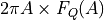$2 \pi A \times F_Q(A)$ vs. the amplitude $A$ . We can regard this product as a work integral, giving the work done by the tip-surface force during the single oscillation cycle of amplitude $A$ (see [Platz-2012b]). For a purely conservative interaction this work is zero at any amplitude. Negative $F_Q$ means that energy in the cantilever was lost via the tip-sample interaction, for example via motion of a viscoelastic surface, or irreversible deformation of the tip or the sample. In contrast, the quantity 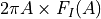$2 \pi A \times F_I(A)$ is not a work integral. If the interaction were described by a conservative force, this quantity is related to the average potential energy change in the oscillation cycle with the amplitude $A$ .

Reconstructed force¶

Sometimes refer to data analysis as inversion , or reconstruction because it involves solving an inverse problem, or reconstructing the force which produced the measured motion, as opposed to forward problem of finding the motion resulting from a given force. As is often the case, the inverse problem is ‘ill-posed’. The limited sensitivity of our measurement gives inadequate information for finding a unique solution to the inverse problem. The very small force that we are trying to determine only gives measurable motion at frequencies in a narrow band close to the high-Q cantilever resonance. Our challenge is therefore to reconstruct the force from this partial spectrum, or narrow band response. Fortunately, with enough intermodulation spectral data, and with a few assumptions that physically well motivated, we can find solutions.

The Force tab brings up a single plot of the effective conservative force vs. cantilever deflection. Zero deflection in this plot corresponds to the equilibrium position, and negative deflection to the cantilever bending toward the surface. In order to reconstruct the force some assumptions about the tip-surface interaction must be made. These assumptions and the different reconstruction methods are described on a separate page:

Force Reconstruction Methods

Force Inspector settings¶

The Settings button in the Force Inspector panel opens a separate panel where you find corresponding tabs to control the different plots and the compensation for background forces. You can also open this panel from the Advanced pull-down menue.

FI FQ and Work tabs have options to Use shading which controls the plotting of the $F_I(A)$ and $F_Q(A)$ curves. When checked (default case) the lightest shade corresponds to the start of the pixel, and the darker shade the end. Use the Signal Inspector and select the Time tab to see the beat-cycle for the selected pixel. With the standard setup, each pixel starts at close to zero amplitude, with increasing amplitude followed by decreasing amplitude. Thus the shading allows you to see how $F_I(A)$ and $F_Q(A)$ differ from increasing to decreasing amplitude.
Force tab contains several options, explained in detail in Force Reconstruction Methods.

Background force compensation¶

The BG Comp tab in the Force Inspector Settings controls background force compensation. The compensation requires measurement of the just-lifted response (see Measure just lifted). If there is not a just-lifted pixel measured, you will get the same result as if None were selected. The theory and application of background force compensation is described in [Borgani-2017].

None turns off the compensation, in which case all force curves will include background forces.
Polynomial fits the linear response function of the background forces to a polynomial in frequency, of the Polynomial degree given. For standard two-drive-frequency ImAFM™, you want to choose the default value polynomial degree = 1 (two points can only determine a straight line). The polynomial of higher degree is only interesting if you use the Drive Constructor to create drive schemes with several drive tones.
Harm. Osc. describes the effect of the background forces as a renormalization of the cantilever parameters f0 and Q.

Note

If you did not make a measurement of the just-lifted response during the scan, it is still possible to perform background compensation. If the scan file has a parachuting pixel somewhere in the image you can use the response at this pixel as the just-lifted response. Select this pixel with the Pixel inspector tool. Open the Data Tree and find the selected pixel in the tree. Right click on that pixel in the tree and choose Redefine as lift oscillation. This redefinition is only temporary. To make it permanent, you must save the .imp file (right click on the file in the tree) possibly with a new file name.

Table of Contents

Previous topic

Next topic

This Page