Force Reconstruction Methods
Force reconstruction can be performed on individual pixels via the Force Inspector, on selected lines in an image by Analyzing Linear Transects, or on entire images via Batch process parameter maps and force volume data.
ImAFM™ reconstructs tip-surface force  as a function of cantilever deflection
  , where the probe height
  and the tip position
  are measured from a fixed position in the inertial reference frame where the sample is at rest (the lab frame). ImAFM™ force measurement is fast enough such that one can assume constant probe height at each pixel. This assumption will however break down when the feedback error signal is large and the base is moving rapidly to compensate for a rapid change in surface topography. ImAFM™ makes no assumption about where the surface actually is in relation to the probe height. This is in stark contrast to quasi static force measurement methods, where one must assume a rigid tip and surface when calibrating the measurement of
  by moving . In fact, ImAFM™ allows you to unambiguously define the location of the surface relative to , by associating it with a distinct feature on the curve (see [Forchheimer-2012]).
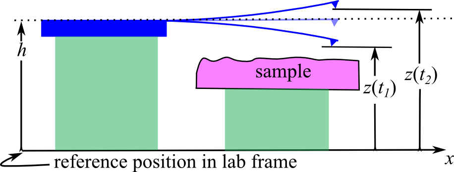
The AFM detector measures cantilever deflection . The probe height is adjusted while scanning. The tip position in the lab frame is  .
.
Three basic methods are available for reconstructing .
In the Force tab of the Force inspector settings panel, check the box to activate the desired Reconstruction Method. You can use any combination of methods, and plot all results on the same plot. Each method makes different assumptions described below. Click the method name to highlight it and view the options for that method.
Polynomial
The Polynomial method approximates the conservative tip-surface force (a function of tip-surface separation only) as a polynomial of finite degree  in the cantilever deflection, .
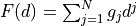
A further assumption is that the force is zero when the tip is sufficiently far from the surface. Under these assumptions we can find the polynomial coefficients  , both odd and even coefficients, from the measured spectrum of odd-order intermodulation products. The method is described in detail in [Platz-2012a], [Platz-2013b].
Polynomial reconstruction has the following options:
line stylegives some plotting options for line type and thickness.Maximum IMP orderis largest order of intermodulation product used in the determination of the polynomial coefficients. High order intermodulation products have lower signal level and depending on your scanning conditions, they will disappear into the noise at some maximum order. The maximum order should be set to the largest order IMP, which has a reasonable signal-to-noise ratio (SNR). You can judge the signal the SNR by simply looking for contrast in the amplitude and phase images of any order IMP.Polynomial degreeis the number of coefficients in the polynomial approximation of the force. This number can not be greater than the maximum order intermodulation product in your spectrum.Assume localized forcecheck-box activates the routine to determine the even polynomial coefficients.Zero force regionsets the crossover deflection , above which the tip-surface force is assumed to be zero. The range is given in normalized coordinates, where -1.0 means closest to the surface, and +1.0 means furthest from the surface. If you uncheck this fitting option you will reconstruct a force curve which is an odd function of deflection,
 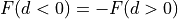 . The odd nature of the curve is due to the fact that the intermodulation spectrum of odd-order products, is only able to reconstruct the polynomial coefficients, with odd
  (see [Platz-2013b]). If this odd curve shows a well developed zero force region for
  , then we can safely neglect long-range forces and the assumption that
  for
for  is well motivated. Move the slider to change .
Model Fit
The Model Fit method assumes that the tip surface force is described by a particular interaction model, which has some number of parameters. The method performs a numerical optimization, adjusting the parameters of the model, so as to best reproduce the measured frequency components of the tip-surface force. The method is described in detail in [Forchheimer-2012], [Forchheimer-2013], [Platz-2012a]. Nearly any model can be fit to the experimental data, so long as it can be coded on a computer. However, the solver will spit out a solution and the software will give you a plot which looks like your force model - even if it is a lousy fit to your data. Model Fit should always be used together with Polynomial or ADFS, in order to independently check if the model makes sense. Model Fit also requires reasonable initial conditions for the solver to converge to a good solution.
Model Fit reconstruction has the following options:
line stylegives some plotting options for line type and thickness.Choose model:selects the different force models that are programed in the software. You can also add your own models to the software, as described in the advanced section on Programming your own Force Models. The help icon opens a window showing the functional form, a list of parameters, and plot of for each model.
The table gives a listing of the parameters for each model, and the initial value for the numerical solver. If the check-box is unchecked, the solver will not adjust that parameter and it will be fixed at it’s initial value.
Model Fit can be applied to every pixel in a scan to generate a parameter map, as described in Batch process parameter maps and force volume data.
Amplitude Dependent Force Spectroscopy (ADFS)
ADFS works from the assumption that it the the force can be written function of the tip position, i.e. there exists a force curve . It further assumes that the force is zero for positive deflection, i.e. for  . If these assumptions are valid, the curve is extracted by performing an inverse Able Transform on the
  curve. The method is described in detail in [Platz-2012b] , [Platz-2013a]. This method can be applied to create a force volume data set from a scan data file, as described in Batch process parameter maps and force volume data.
Three features control ADFS:
Reconstruct from FI(A) for:is a pull-down menu selector that allows you to select different regions of the curve that will be used for ADFS. Usually best results are found for longest monotonous amplitude increasewhich is the default selection. However, you can reconstruct for decreasing amplitude, or for a mean curve, which averages the increasing and decreasing amplitude. Note that often with soft materials, the and  show hysteresis, meaning that they are different for increasing or decreasing amplitude. This can be a sign that the surface is not relaxing to its equilibrium position between successive taps of the tip. In this case a force curve can not describe the interaction, and ADFS gives only an approximate view of the force.
Stavitzky - Golay smoothingis a routine to smooth the ADFS force curves. Smoothing supresses wiggles in the force curves, caused by noise and limited spectral range of the cantilever. Two numbers control the smoothing: Thesmoothing window length [%]is the precent of the total number of points in the full force curve, over which the smoothing is made. You can also choose theSmoothing polynomial degree. The smoothing fits a polynomial over a sliding window, to generate a smoothed point.
Fast Polynomial
A computationally efficient method to determine the polynomial coefficients of the conservative tip-surface force is described in [Platz-2013b]. The method is very fast compared to standard Polynomial and Model Fit. The faster computation enables parameter mapping in real time, as scan data is acquired.
Live parameter mapping available as a script the pull-down menu: Advanced -> Scripts -> LiveParameterMap.
Startwill activate this feature and you can see the selectedParameteras a color map, painted during the scan.Show force curvewhen activated will plot the polynomial force curve at the center pixel of every scan line. The force plot displays the selected parameter with a line or point on the force curve.
This type of parameter map can also be applied to scan data file, as described in Batch process parameter maps and force volume data.